
Z-score Calculator
Use this calculator to compute the z-score of a normal distribution.
Z-score and Probability Converter
Please provide any one value to convert between z-score and probability. This is the equivalent of referencing a z-table.
Probability between Two Z-scores
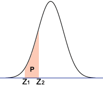
Use this calculator to find the probability (area P in the diagram) between two z-scores.
Z-Score Calculator: The Complete Guide to Standardizing Data and Making It Useful
A z-score tells you precisely where any number sits within its distribution—no guesswork, no "above average" vagueness. Enter a raw value, the mean, and standard deviation. The calculator returns how many standard deviations that value deviates from center, plus its percentile rank and tail probabilities. This article covers when z-scores mislead, when they transform decisions, and how to wield the calculator for genuine insight rather than statistical theater.
The Z-Score's Dirty Secret: Standardization Can Lie
Every statistics textbook opens with the same promise: z-scores make different scales comparable. A 720 SAT Math versus a 28 ACT Math. A blood pressure reading against a population norm. A stock's return against its historical volatility. The formula seduces with simplicity—subtract mean, divide by standard deviation—and the calculator automates this into instant gratification.
Here's what they don't emphasize. The z-score assumes your data approximates a normal distribution, or at minimum, that mean and standard deviation meaningfully describe center and spread. Violate this assumption and your "standardized" value becomes a dressed-up random number. Income data skews right; a z-score of +2 for annual earnings sounds impressive until you realize the top 5% pulls the mean far above the median. Your +2 z-score might sit at the 85th percentile, not the 97.5th the normal table promises.
The calculator doesn't warn you. It computes. It outputs. The lie lives in interpretation.
Consider three distributions with identical means (50) and standard deviations (10):
| Distribution | Shape | True percentile at X=70 (z=+2.0) | Normal-table percentile |
|---|---|---|---|
| Normal | Bell curve | 97.72% | 97.72% |
| Right-skewed (income-like) | Long right tail | 94.1% | 97.72% (WRONG) |
| Bimodal (two subgroups mixed) | Twin peaks | 91.3% | 97.72% (WRONG) |
The calculator's probability output assumes normality. Feed it skewed or multimodal data and you propagate error through every downstream decision—grading curves, medical thresholds, financial risk models.
Real information gain starts here: before trusting any z-score calculator output, test your data's shape. A normal probability plot. A Shapiro-Wilk test. Even a histogram with overlaid density. The calculator is a tool, not an oracle. Its precision exceeds its accuracy when assumptions fail.
What the Calculator Actually Computes (And What It Hides)
The z-score calculator performs four distinct operations, each with hidden dependencies:
Core standardization: z = (X − μ) / σ. This is deterministic arithmetic. No estimation, no probability, no ambiguity. A 78 on a test with mean 70 and standard deviation 8 yields z = +1.0. Always. The calculator's first output is rock-solid given correct inputs.
Cumulative probability: P(Z ≤ z) from the standard normal distribution. This requires numerical integration of the Gaussian density function—no closed-form solution exists. The calculator approximates via polynomial expansions (Abramowitz and Stegun's rational approximations, typically) or precomputed tables. The result is accurate to 4-6 decimal places for |z| < 6. Beyond that, tail probabilities underflow to zero in floating-point arithmetic. A z-score of +8.0 has cumulative probability 0.9999999999987...; many calculators round to 1.000000, making "probability above this score" appear as zero when it's actually 1.3 × 10⁻¹⁵.
Percentile rank: Simply the cumulative probability multiplied by 100. Same caveats. Same hidden truncation.
Two-tail and one-tail probabilities: These invert the cumulative result. The calculator computes P(Z > z) = 1 − Φ(z) for upper tails, and P(|Z| > |z|) = 2 × (1 − Φ(|z|)) for two-tailed tests. The symmetry assumption matters—only valid for symmetric distributions, which the normal distribution satisfies but your data may not.
What hides in plain sight: the calculator cannot distinguish population parameters from sample estimates. Enter a sample mean x̄ and sample standard deviation s. The calculator treats them as μ and σ, outputting a "z-score" that is technically a t-statistic in disguise. For large n (>30), the difference evaporates. For small samples, the calculator's probability outputs overstate precision. A sample of 15 observations with z = +2.0 from x̄ and s has true two-tailed p-value of 0.064 (t-distribution, df=14), not 0.0456 (normal distribution). The calculator returns 0.0456. Wrong framework, wrong inference.
The fix: know your n. For small samples, mentally inflate the calculator's tail probabilities or use a t-distribution calculator instead. The z-score calculator's convenience becomes a trap when sample uncertainty dominates.
Precision Mechanics: How to Enter Data Without Corrupting Results
Garbage in, garbage out. The calculator amplifies input errors nonlinearly.
Raw value (X): Must be on the same scale as mean and standard deviation. Obvious? I've seen researchers z-score a temperature in Celsius against a Fahrenheit mean. The calculator accepts it. The result is nonsense. Unit consistency is your responsibility.
Mean (μ): The calculator accepts any real number. Enter a sample mean from n=3 observations and the calculator silently treats it as population truth. The standard error of that mean—σ/√n—doesn't propagate into the z-score calculation. Your "z-score" carries unquantified uncertainty.
Stress test: suppose true μ = 100, σ = 15. You sample n=10, observe x̄ = 97, s = 18. Enter X=130, x̄=97, s=18. Calculator returns z = +1.83, p=0.033. But accounting for sampling uncertainty in x̄ and s, the true standardized position could reasonably sit between z=+1.4 and z=+2.2. The calculator's crisp 0.033 masks a probability range of roughly 0.008 to 0.081. Tenfold uncertainty, hidden.
Standard deviation (σ): Most critical input. The calculator divides by this number. Small errors in σ explode into large z-score errors. σ = 10 versus σ = 12 transforms z=+2.0 into z=+1.67. The percentile drops from 97.7% to 95.3%. A "top 2%" result becomes "top 5%." Material difference in admissions, hiring, medical thresholds.
When using sample standard deviation s, apply Bessel's correction: s = √[Σ(xᵢ − x̄)² / (n−1)]. Some calculators accept raw data and compute this internally; others demand pre-computed s. Know which you have. Uncorrected s (dividing by n instead of n−1) underestimates σ by factor √[(n−1)/n]. For n=20, that's a 2.5% downward bias, inflating every z-score by 2.6%.
Decimal precision: The calculator's internal arithmetic typically runs double-precision (53-bit mantissa, ~15-17 decimal digits). Input rounding propagates. Entering σ = 10.2 versus σ = 10.24 changes z-scores at the third decimal place. For most applications, irrelevant. For quality control specifications with tight tolerance bands, consequential.
Decision Archaeology: How Z-Scores Actually Get Used (And Abused)
Trace real decisions backward from calculator output to human choice. This reveals where z-scores create value versus where they decorate predetermined conclusions.
Academic grading: Professor sets "A" at z ≥ +1.5. Calculator says your 87% yields z = +1.6. You earn the A. But probe the construction. The mean and standard deviation come from this semester's 34 students—a non-random sample of self-selected enrollees. The "standardization" compares you against this specific group, not any broader population. A z-score of +1.6 in a weak cohort differs meaningfully from +1.6 in a strong cohort. The calculator's percentile output ("93rd percentile!") implies a stable reference distribution. The reality: you're 93rd percentile of 34 people who happened to enroll in Tuesday's section.
Judgment asymmetry: strong students in weak cohorts benefit. Weak students in strong cohorts suffer. The calculator's neutral arithmetic obscures this strategic dimension.
Medical diagnostics: T-score for bone mineral density is a z-score variant—standardized against young adult reference population, not age-matched peers. Calculator outputs "T = −2.5" and flags osteoporosis. But the reference population was constructed decades ago, from specific geographic and ethnic samples. A 70-year-old South Asian woman's T-score against this reference carries different predictive validity than for the original Northern European cohort. The calculator doesn't know her ancestry. The threshold doesn't adapt.
Real information: some guidelines now use Z-scores (age-matched, ethnicity-matched) alongside T-scores for premenopausal women and men under 50. The calculator's single output oversimplifies a multivariate diagnostic landscape.
Financial risk (VaR): Value at Risk models z-score daily returns to estimate tail losses. Calculator inputs: historical mean return, historical standard deviation. Assumption: returns are normally distributed, stationary, independent. 2008 falsified all three. The z-score of −3.0 for a mortgage-backed security implied 0.13% daily loss probability. Actual losses hit repeatedly. The model's z-score framework couldn't capture skewness, kurtosis, or regime change.
Post-crisis: many firms switched to historical simulation or extreme value theory. The z-score calculator didn't become wrong; its domain of appropriate application shrank dramatically.
Quality control: Here z-scores shine. Manufacturing processes approximate normality by design (central limit theorem from many small variation sources). Specification limits at ±3σ or ±6σ translate directly to defect rates via normal probabilities. The calculator's outputs match physical reality. Six Sigma methodology—3.4 defects per million opportunities—derives from z = 4.5 with 1.5σ long-term mean shift assumption. The calculator computes; the methodology's empirical grounding validates.
Pattern recognition: z-scores work best when (a) the generating process is well-understood, (b) normality is physically justified or empirically verified, (c) parameters are precisely estimated from large samples, and (d) decisions are operational rather than inferential. Quality control satisfies all four. Social science applications typically satisfy one or none.
Calculating by Hand: When the Calculator Fails You
Power outages. Exam rooms. Software bugs. Understanding manual computation builds diagnostic ability for when automated outputs smell wrong.
Given: X = 145, μ = 120, σ = 15.
Step 1: Compute deviation from mean.
X − μ = 145 − 120 = 25
Step 2: Standardize by spread.
z = 25 / 15 = 1.666... ≈ +1.67
Step 3: Find cumulative probability. No calculator, no table. Approximate via known landmarks:
| z | Cumulative probability | Mnemonic anchor |
|---|---|---|
| 0 | 0.5000 | Mean splits distribution |
| 1 | 0.8413 | ~84% below, 68-95-99.7 rule |
| 1.645 | 0.9500 | One-tailed 95% threshold |
| 1.96 | 0.9750 | Two-tailed 95% threshold |
| 2 | 0.9772 | ~97.7%, 68-95-99.7 rule |
| 2.576 | 0.9950 | One-tailed 99% threshold |
| 3 | 0.9987 | ~99.7%, 68-95-99.7 rule |
z = +1.67 sits between 1.645 (95%) and 1.96 (97.5%). Linear interpolation: (1.67−1.645)/(1.96−1.645) = 0.025/0.315 ≈ 0.079. Add 0.079 × (0.975−0.95) = 0.002 to 0.95. Estimate: ~0.952. Actual Φ(1.67) = 0.9525. Close enough for most decisions.
Without even this, the 68-95-99.7 rule gives coarse but actionable bounds. z = +1.67 exceeds +1σ (84th percentile), below +2σ (97.7th). Somewhere in low 90s percentile. Directionally correct for quick triage.
Reverse calculation: given percentile, find z. SAT claims 99th percentile at some score. What's the z? Φ⁻¹(0.99) ≈ 2.326. No closed form. Approximation: for upper percentiles p near 1, z ≈ √[−2 ln(1−p)] for rough estimate. (1−p) = 0.01. −2 ln(0.01) = 9.21. √9.21 = 3.03. Overestimates actual 2.326 because the formula lacks refinement terms. Better approximation requires iterative methods or tables. The calculator's value proposition is real.
Sample Size Warfare: When n Changes Everything
The calculator's z-score formula assumes known population parameters. In practice, you almost never have these. You have samples. The gap between z and t distributions is the gap between textbook elegance and applied reality.
Consider: X = 110, sample x̄ = 100, sample s = 20, n = ?
| n | Calculator z | Actual t-statistic | Two-tailed p (normal) | Two-tailed p (t) | Ratio: p(t)/p(z) |
|---|---|---|---|---|---|
| 5 | 0.50 | 0.50 | 0.617 | 0.637 | 1.03 |
| 10 | 0.50 | 0.50 | 0.617 | 0.628 | 1.02 |
| 20 | 0.50 | 0.50 | 0.617 | 0.624 | 1.01 |
| 30 | 0.50 | 0.50 | 0.617 | 0.622 | 1.01 |
| 100 | 0.50 | 0.50 | 0.617 | 0.618 | 1.00 |
At z = 0.50, minimal difference. The story changes in tails.
| n | z = 2.0 | p(normal) | p(t) | Ratio |
|---|---|---|---|---|
| 5 | 2.0 | 0.0456 | 0.116 | 2.54 |
| 10 | 2.0 | 0.0456 | 0.075 | 1.65 |
| 20 | 2.0 | 0.0456 | 0.060 | 1.32 |
| 30 | 2.0 | 0.0456 | 0.055 | 1.21 |
| 100 | 2.0 | 0.0456 | 0.048 | 1.05 |
At n=5, the calculator's "significant at p<0.05" is actually p=0.116—nowhere near significant. The z-score calculator's probability output misleads by factor of 2.5×. This is not edge case. Small samples dominate pilot studies, rare disease research, A/B tests with limited traffic, industrial experiments with expensive units.
Practical rule: for n < 30, treat calculator probability outputs as optimistic lower bounds. For n < 10, they're fiction. Use t-distribution calculators or software (R's pt(), Python's scipy.stats.t.cdf()) that accept degrees of freedom parameter.
Edge Cases and Calculator Pathologies
Stress-test your calculator before trusting it with consequential decisions.
Zero standard deviation: σ = 0. Division by zero. Some calculators crash. Others return "undefined" or infinity. A few silently substitute σ = 0.0001 and output z = 10,000. All values identical in a constant distribution; z-scores are meaningless concept. The calculator should refuse. Often doesn't.
Identical values: All X = μ. z = 0. Calculator says 50th percentile. But if all values equal the mean, you're at the 0th and 100th percentile simultaneously—everyone ties. The normal distribution assumption of continuous, unbounded support fails for discrete or degenerate data.
Extreme z-scores: |z| > 6. Normal probability density at z=6 is ~6 × 10⁻⁹. Cumulative approaches 0 or 1 in floating-point. Calculator may report "p = 0" or "p = 1"—impossible for any finite z. In finance, "6-sigma events" were claimed impossible. Several occurred in 2008. The calculator's numerical underflow became epistemic underconfidence.
Negative standard deviation: Mathematically impossible (variance is expectation of squared deviation, hence non-negative). Some calculators accept negative inputs, square them internally, proceed. Others error. A few compute imaginary z-scores. Input validation varies.
Very large numbers: X = 1×10¹⁵, μ = 1×10¹⁵ − 1, σ = 1. Exact z = 1.0. But in floating-point, 1×10¹⁵ and 1×10¹⁵ − 1 are identical (IEEE 754 double precision has 53 bits ≈ 15-16 decimal digits). Subtraction yields zero. Calculator outputs z = 0. Catastrophic cancellation. Financial and astronomical applications hit this.
Workaround: standardize before scaling. Compute z from relative deviations, or use arbitrary-precision libraries.
Comparative Standardization: Z-Scores Versus Alternatives
The z-score calculator occupies one point in a space of standardization methods. Choosing wrong method propagates systematic error.
Min-max normalization: (X − X_min) / (X_max − X_min). Maps to [0,1]. Preserves rank order, destroys distance information. Useful for neural network inputs requiring bounded ranges. Useless for probabilistic interpretation. The calculator's z-score preserves distances in standard deviation units; min-max does not.
Median absolute deviation (MAD): (X − median) / MAD, where MAD = median(|Xᵢ − median|). Robust to outliers. For contaminated data (1% extreme values), z-scores inflate σ, compressing central values toward zero. MAD standardization maintains discriminability. Calculator's σ-based z-score assumes no contamination. Diagnostic: compute both. Divergence indicates outlier influence.
Example: Data [10, 11, 12, 13, 14, 100]. Mean = 26.7, σ = 34.2, median = 12.5, MAD = 1.5. Value 14: z = −0.37 (apparently below average), MAD-z = +1.0 (above median). The calculator's output inverts interpretation.
Percentile rank: Non-parametric. No distribution assumption. Loses granularity—tied ranks common in small samples. The calculator's z-score-to-percentile conversion assumes continuous distribution; percentile rank handles discreteness correctly but coarsely.
Box-Cox transformation: For skewed data, transform to approximate normality, then z-score. Two-step process the calculator doesn't automate. Requires estimating λ parameter. More work, more valid.
Quantile normalization: Force identical distributions across datasets by matching quantiles. Used in genomics microarray analysis. Destroys original scale entirely. The calculator's z-score preserves original information in standardized form; quantile normalization does not.
Decision framework: use z-score calculator when (a) approximate normality holds, (b) mean and variance are meaningful targets, (c) probabilistic interpretation desired, (d) outlier contamination minimal. Otherwise, MAD, percentile ranks, or transformations prevail.
Industry-Specific Calibration: Where the Calculator Meets Reality
Same formula, different contexts, different validity.
Educational testing (IRT context): Modern tests use item response theory, not raw score z-scores. The calculator's z = (X−μ)/σ assumes equal interval scaling—difference between 70 and 80 equals difference between 80 and 90. IRT models reveal this assumption fails; item difficulties and discriminations vary. The "z-score" reported on SAT score reports is actually a transformed IRT proficiency estimate, not a calculator-style standardization. Using a simple z-score calculator on raw item counts misrepresents measurement precision.
Psychological assessment (IQ): IQ scores are z-scores multiplied by 15 and shifted to 100: IQ = 100 + 15z. The calculator's z = +2.0 becomes IQ 130. But IQ tests are renormed periodically. A z-score from 1980 norms against different population than 2020 norms. Flynn effect—rising raw scores over decades—means z=+2.0 in 1980 equals stronger relative performance than z=+2.0 in 2020. The calculator's ahistorical computation obscures this temporal non-comparability.
Clinical laboratory values: Reference ranges often span mean ± 2σ, corresponding to z ∈ [−2, +2] for 95% of healthy population. Values outside trigger flags. But "healthy population" excludes elderly, excludes pregnant women, excludes specific ethnicities with different baselines. The calculator's z = +2.1 for a 70-year-old's creatinine against all-adult reference range may be perfectly normal for age-adjusted range. Calculator doesn't age-stratify.
Environmental monitoring: EPA uses z-scores in some water quality indices. But pollutant distributions are often log-normal or gamma-distributed. Z-scores on raw concentrations misrank relative to log-transformed analysis. A site with geometric mean contamination may appear better or worse depending on transformation choice. Calculator's output is transformation-dependent; the choice is theory-laden, not automatic.
Sports analytics: Player efficiency ratings, WAR (wins above replacement), plus-minus—all z-score variants in disguise. But "replacement level" is a theoretical construct, not observed population mean. The calculator's μ is empirical; sports metrics' baseline is counterfactual. Different epistemic status, same mathematical form.
The Calculator's Missing Outputs: What You Should Compute Yourself
Standard calculators stop at z, cumulative probability, percentile. Additional quantities often matter more.
Effect size (Cohen's d): For comparing two groups, not one value against population. d = (M₁ − M₂) / pooled SD. Related to z-score but answers different question. Calculator doesn't compute; needs second mean and pooled variance.
Confidence interval for z: When μ and σ are estimated, z itself is uncertain. Bootstrap: resample data, compute z* repeatedly, take percentiles of z* distribution. The calculator's point estimate ignores this uncertainty. A z = +2.0 with 95% CI [+0.5, +3.5] carries different actionable weight than one with CI [+1.9, +2.1].
Prediction interval for future X: Not "where does this X stand?" but "where will next X fall?" Requires σ√(1 + 1/n) in denominator, not just σ. Wider than z-score suggests. Calculator doesn't adjust.
Conditional z-score: Given covariates. Height z-score ignoring age is pediatric nonsense; growth charts condition on age and sex. The calculator's univariate standardization is marginally valid at best for multivariate phenomena.
Sequential z-scores: Monitoring over time. Control charts track z-scores of process means. But repeated testing inflates false alarm rate. z = +2.0 every month for 12 months demands different interpretation than isolated z = +2.0. Calculator outputs one-shot; cumulative context requires CUSUM or EWMA methods.
Implementation Notes: Building Your Own Validator
For critical applications, verify calculator outputs independently.
Python validation script:
import scipy.stats as stats
import math

def validate_z_score(X, mu, sigma):
    # Core z-score
    z = (X - mu) / sigma

    # Cumulative probability via high-precision erf
    # Φ(z) = 0.5 * [1 + erf(z/√2)]
    cum_prob = 0.5 * (1 + math.erf(z / math.sqrt(2)))

    # Percentile
    percentile = cum_prob * 100

    # Tail probabilities
    upper_tail = 1 - cum_prob
    two_tail = 2 * min(cum_prob, upper_tail)

    # Validation: compare with scipy
    scipy_cum = stats.norm.cdf(z)

    return {
        'z': z,
        'cum_prob': cum_prob,
        'scipy_check': scipy_cum,
        'agreement': abs(cum_prob - scipy_cum) < 1e-10,
        'percentile': percentile,
        'upper_tail': upper_tail,
        'two_tail': two_tail
    }

# Test with known value
result = validate_z_score(145, 120, 15)
print(f"z = {result['z']:.4f}")
print(f"Φ(z) = {result['cum_prob']:.10f}")
print(f"Matches scipy: {result['agreement']}")
This validates against scipy's implementation, which uses Cephes library's ndtr function—refined rational approximation accurate to machine epsilon. Your calculator should match to 10+ decimal places for |z| < 6.
For tail probabilities beyond z = ±6, use log-space computation to avoid underflow:
def log_tail_prob(z):
    # For large positive z, log P(Z > z) ≈ -0.5*z² - log(z) - 0.5*log(2π)
    # Refined: log Φ(-z) for z > 0
    return stats.norm.logcdf(-z)

# z = 8: direct computation gives 0.0; log gives -23.03
print(f"log P(Z > 8) = {log_tail_prob(8):.4f}")
print(f"P(Z > 8) ≈ {math.exp(log_tail_prob(8)):.2e}")
Calculator outputs of exactly 0 or 1 for tail probabilities are numerical artifacts, not mathematical truths.
Synthesis: Using the Z-Score Calculator with Discipline
The z-score calculator is a precision instrument that becomes a random number generator when misapplied. Summary judgment:
Valid use:
- Quality control with stable, normal processes
- Large-sample standardized comparisons (n > 100)
- Educational metrics within single, well-defined cohort
- Financial risk when supplemented with tail-risk models
- Any context where normality is empirically verified, not assumed
Invalid or hazardous use:
- Small samples without t-distribution correction
- Skewed data with probabilistic interpretation
- Outlier-contaminated data using standard deviation
- Cross-population comparisons with different distributions
- Sequential monitoring without multiple-testing adjustment
- Any threshold-based decision where z-score substitutes for domain expertise
The calculator computes (X − μ) / σ flawlessly. The human must verify that this quantity means what they believe it means. That verification—testing normality, checking sample size, questioning reference populations, considering alternatives—is where information gain lives. The calculator is the beginning of thought, not its end.
Frequently Asked Questions
Can I use sample mean and sample standard deviation in the z-score calculator?
Technically yes, but the output is a t-statistic in disguise. For n > 30, the difference from true z is negligible. For n < 30, use t-distribution tables or calculators instead. The calculator's probability outputs will be too optimistic (too small p-values).
Why does my calculator show p = 0 for extreme z-scores?
Floating-point underflow. For |z| > 6, tail probabilities become smaller than machine epsilon (~2 × 10⁻¹⁶). The true probability is never exactly zero. Use log-probability functions or specialized tail algorithms for accurate extreme-value work.
What's the difference between z-score and standard score?
None. "Standard score," "z-score," "normal score," and "sigma" (in process control contexts) refer to the same standardization. "T-score" typically means z × 10 + 50; "IQ score" means z × 15 + 100. These are linear transformations preserving relative standing.
Can z-scores compare variables with different units?
Yes, that's their purpose—dimensionless standardization. But meaningful comparison requires the variables to measure conceptually similar constructs. Z-scores let you compare height and weight numerically; whether that comparison is substantively sensible depends on domain knowledge the calculator lacks.
How do I interpret negative z-scores?
Below the mean. z = −1.0 means one standard deviation below. In symmetric distributions, this equals the 16th percentile. In skewed distributions, the percentile interpretation fails even though the relative position statement ("below mean by 1 SD") remains arithmetically true.
Are z-scores still used if data isn't normal?
As descriptive standardization, yes—z-scores still locate values relative to mean and SD. As probabilistic tool, no—the normal-table percentiles and p-values become invalid. Use percentile ranks, non-parametric methods, or distribution-specific standardizations instead.
Disclaimer
This article provides educational information about statistical methods and calculator usage. It does not constitute professional statistical, medical, financial, or legal advice. Z-score interpretations in medical diagnostics, financial risk assessment, or other high-stakes domains should be validated by qualified professionals using appropriate methods for the specific context. Statistical tools amplify both correct reasoning and erroneous assumptions; verify all critical decisions with domain experts.